ex1-linear regression
AndrewNg 机器学习习题ex1-linear regression
练习用数据
练习数据ex1data1.txt和ex2data2.txt都是以逗号为分割符的文本文件,所以我们也可以把它们看作csv文件处理。
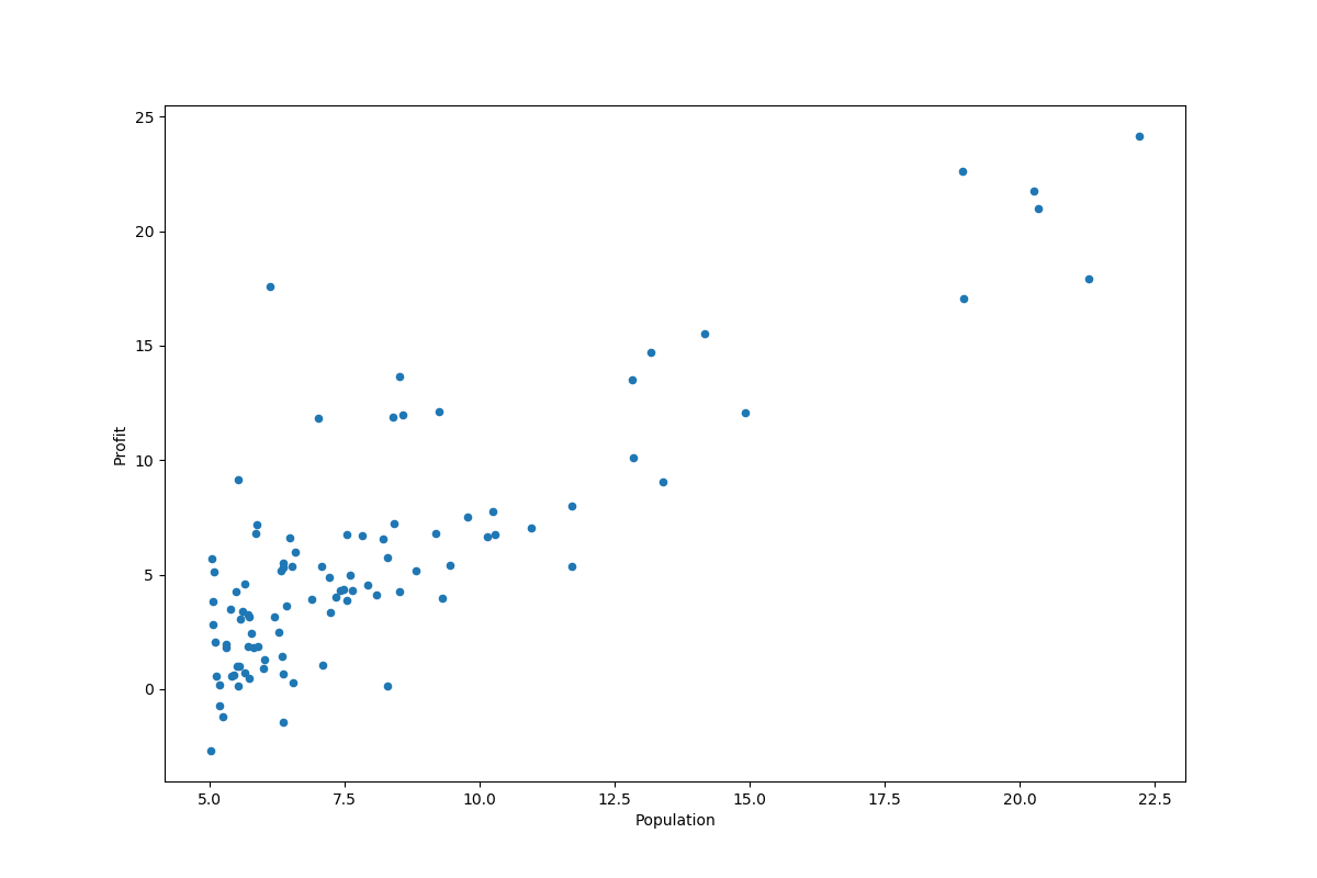
ex1data1中的第一列是一个城市的人口,第二列是这个城市中卡车司机的利润。
ex2data2三列分别是,一个房子的大小,房间数,售价。
浏览数据
import numpy as np
import pandas as pd
import matplotlib.pyplot as plt

# 加载数据
path = './data/ex1data1.txt'
data = pd.read_csv(path, header=None, names=['Population', 'Profit'])
# 看一下数据的内容
print(data.head())
print(data.describe())
# 画出散点图
data.plot(kind='scatter', x='Population', y='Profit', figsize=(12, 8))
plt.show()
| - | Population | Profit |
|---|---|---|
| 0 | 6.1101 | 17.5920 |
| 1 | 5.5277 | 9.1302 |
| 2 | 8.5186 | 13.6620 |
| 3 | 7.0032 | 11.8540 |
| 4 | 5.8598 | 6.8233 |
| - | Population | Profit |
|---|---|---|
| count | 97.000000 | 97.000000 |
| mean | 8.159800 | 5.839135 |
| std | 3.869884 | 5.510262 |
| min | 5.026900 | -2.680700 |
| 25% | 5.707700 | 1.986900 |
| 50% | 6.589400 | 4.562300 |
| 75% | 8.578100 | 7.046700 |
| max | 22.203000 | 24.147000 |
代价函数
我们将创建一个以参数θ为特征函数的代价函数
其中:
def compute_cost(X, y, theta):
    inner = np.power(((X * theta.T) - y), 2)
    return np.sum(inner) / (2 * len(X))
预处理
# 预处理
data.insert(0, 'Ones', 1)  # 添加一列1
cols = data.shape[1]
X = data.iloc[:, :cols - 1]  # 去掉最后一列
Y = data.iloc[:, cols - 1: cols]  # 最后一列

# 检查X和Y 是否正确
print(X.head())
print(Y.head())

# 把X和Y转换为numpy的矩阵
X = np.matrix(X.values)
Y = np.matrix(Y.values)
# 初始化theta
theta = np.matrix(np.array([0, 0]))
# 检查维度
print(X.shape, Y.shape, theta.shape)  # (97, 2) (97, 1) (1, 2)
批量梯度下降
我们要这个公式来更新θ。
# 梯度下降
# X矩阵,Y矩阵,初始的θ,学习速率,迭代次数
def gradient_descent(X, Y, theta, alpha, iters):
    temp = np.matrix(np.zeros(theta.shape))
    parameters = int(theta.ravel().shape[1])
    cost =  np.zeros(iters)

    for i in range(iters):
        error = (X * theta.T) - Y
        for j in range(parameters):
            term = np.multiply(error, X[:, j])
            temp[0, j] = theta[0, j] - ((alpha / len(X)) * np.sum(term))
        theta = temp
        cost[i] = compute_cost(X, Y, theta)

    return theta, cost


# 初始化迭代次数和学习速率
alpha = 0.01
iters = 1000

g, cost = gradient_descent(X, Y, theta, alpha, iters)
# 用我们得到的参数g计算代价函数,查看误差
print(g, compute_cost(X, Y, theta))
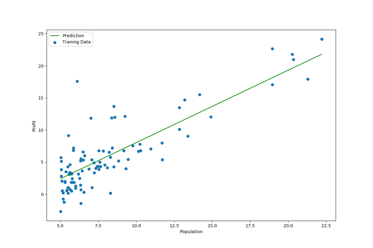
可视化
# 绘制线性模型以及数据,查看拟合效果
def data_visual(data, g):
    x = np.linspace(data.Population.min(), data.Population.max(), 100)
    f = g[0, 0] + (g[0, 1] * x)

    fig, ax = plt.subplots(figsize=(12, 8))
    ax.plot(x, f, 'g', label='Prediction')
    ax.scatter(data.Population, data.Profit, label='Traning Data')
    ax.legend(loc=2)
    ax.set_xlabel('Population')
    ax.set_ylabel('Profit')
    plt.show()

data_visual(data, g)
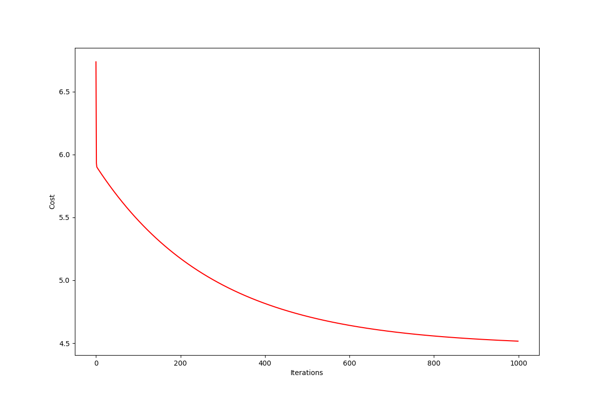
# 绘制代价向量
def cost_visual(cost):
    fig, ax = plt.subplots(figsize=(12, 8))
    ax.plot(np.arange(iters), cost, 'r')
    ax.set_xlabel('Iterations')
    ax.set_ylabel('Cost')
    plt.show()

cost_visual(cost)
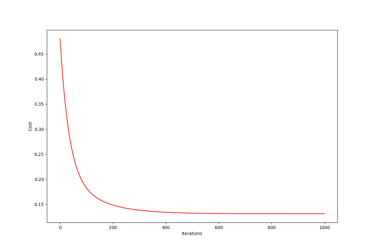
多变量的线性回归
练习1还包括一个房屋价格数据集,其中有2个变量(房子的大小,卧室的数量)和目标(房子的价格)。 我们使用我们已经应用的技术来分析数据集。
path = './data/ex1data2.txt'
data2 = pd.read_csv(path, header=None, names =['Size', 'Bedrooms', 'Price'])
print(data2.head())

# 特征归一化
data2 = (data2 - data2.mean()) / data2.std()

# 预处理
# add ones column
data2.insert(0, 'Ones', 1)

# set X (training data) and y (target variable)
cols = data2.shape[1]
X2 = data2.iloc[:, : cols - 1]
Y2 = data2.iloc[:, cols - 1: cols]

# convert to matrices and initialize theta
X2 = np.matrix(X2.values)
Y2 = np.matrix(Y2.values)
theta2 = np.matrix(np.array([0, 0, 0]))

g2, cost2 = gradient_descent(X2, Y2, theta2, alpha, iters)
cost_visual(cost2)
| - | Size | Bedrooms | Price |
|---|---|---|---|
| 0 | 2104 | 3 | 399900 |
| 1 | 1600 | 3 | 329900 |
| 2 | 2400 | 3 | 369000 |
| 3 | 1416 | 2 | 232000 |
| 4 | 3000 | 4 | 539900 |
正规方程
# 正规方程
def normal_func(X ,Y):
    theta = np.linalg.inv(X.T@X)@X.T@Y
    return theta

g = normal_func(X, Y)
data_visual(data, g.T)